

Build a Neural Network with TensorFlow
TensorFlow
In this Project we’ll be using TensorFlow to program and train our own neural network. TensorFlow is a library developed by Google with the soul purpose of accelerating and simplifying the process of building and training machine learning models. As you might have seen in the previous project, Building a Neuron in Python, creating even a single neuron can be a bothersome and complicated task for a beginner. However, libraries such as TensorFlow facilitate the process giving you more room to build more complex models, you’ll see why here in a second.
TensorFlow setup
In a Python IDE(my favorite is pycharm with the anaconda enviroment plugin) import tensorflow as tf. Rarely will you ever see TensorFlow imported as something other than tf unless a specific attribute is being imported.
import tensorflow as tf
Unlike many other machine learning modules, TensorFlow has everything that numpy can do built into it. This tight integration rids us of many type errors since we’ll being using TensorFlow data types along side TensorFlow methods. For example, instead of using a Numpy array we can use tensors which are a special type of multidimensional array unique to TensorFlow, tensors can be a single value, a list, or a multidimensional list of values.
- Since machine learning uses massive datasets and plots them on a graph sometimes the graphs are not fully cleared. Lucky for us, TensorFlow has a built in function for wiping all data that may be crowding our graph:
import tensorflow as tf
tf.reset_default_graph()
Using this function should be the first thing you do before every model. Now time to familiarize ourselves with some of the basic functionalities in TensorFlow. To begin, you can create a constant tensor variable using tf.variable_type(value, dtype = datatype). For this example we’ll create a constant tensor to keep it simple:
import tensorflow as tf
tf.reset_default_graph()
number = tf.constant(50.0, dtype=tf.float32)
The constant part is specifying the type of variable we want to create, which in our case is a constant, 50.0 is the variable value, and float32 is specifying that our value(s)(50.0) equals a float data type. You’ll probably see float32 as the data type for almost every tensor. Before we can do any operations to our constant or to anything for that matter, we have to start a TensorFlow session.
import tensorflow as tf
tf.reset_default_graph()
number = tf.constant(50.0, dtype=tf.float32)

with tf.Session() as sess:
This begins our sessions under the name of sess. I renamed it to sess so we can run operations easily in the session. To show you lets add 20.0 to our constant:
import tensorflow as tf
tf.reset_default_graph()
number = tf.constant(50.0, dtype=tf.float32)

with tf.Session() as sess:
    print(sess.run(number + 20.0))
You might see a few warnings that look like errors, don’t worry, as long as at the end of your console you see an output of “70.0”.
Passing in Input Data
When passing input data into a computational graph, TensorFlow uses placeholders to take in this data. By adjusting the parameters of the placeholder nodes you can change the type of input data that is fed into the graph or network. Every placeholder node has some sort of parameters for shape, shape is the number of dimensions and elements a tensor has. For example, [1,2,3] is one dimension with 3 elements(3), [[1,2],[3,4]] is 2 dimensions with 2 elements per dimension(2,2). Lets create a variable for placeholder input data in the same format that we made the constant variable:
import tensorflow as tf
tf.reset_default_graph()
number = tf.constant(50.0, dtype=tf.float32)
input_node = tf.placeholder(dtype=tf.float32, shape=None)

with tf.Session() as sess:
    print(sess.run(number + 20.0))
Setting the shape parameter equal to None means that the node will take in any input regardless of the shape. To test out the input node, lets multiply whatever passes through it by 2:
import tensorflow as tf
tf.reset_default_graph()
number = tf.constant(50.0, dtype=tf.float32)
input_node = tf.placeholder(dtype=tf.float32, shape=None)

multiply = input_node * 2

with tf.Session() as sess:
    print(sess.run(number + 20.0))
If you try to run the multiply operation right now you would probably get an error because we haven’t passed any data into the input node. We pass data into the input node using the feed_dict parameter:
import tensorflow as tf
tf.reset_default_graph()
number = tf.constant(50.0, dtype=tf.float32)
input_node = tf.placeholder(dtype=tf.float32, shape=None)

multiply = input_node * 2

with tf.Session() as sess:
    print(sess.run(number + 20.0))
    print(sess.run(multiply, feed_dict={input_node: 45.0}))
As you can see we’re feeding 45 into the input_node and multipying it. Since we specified the input shape as none it can take any shape we pass into it.
import tensorflow as tf
tf.reset_default_graph()
number = tf.constant(50.0, dtype=tf.float32)
input_node = tf.placeholder(dtype=tf.float32, shape=None)

multiply = input_node * 2

with tf.Session() as sess:
    print(sess.run(number + 20.0))
    print(sess.run(multiply, feed_dict={input_node: 45.0}))
    print(sess.run(multiply, feed_dict={input_node: [[3, 3], [4, 4], [5, 5]]}))
If you passed in the same (3,3) shape as me you should have received the output:
[[ 6.  6.]
 [ 8.  8.]
 [10. 10.]]
Every element was multiplied by 2. Having the ability to change massive data sets is a crucial part of Machine Learning.
Making the Machine Learning Model:
For this Project the neural network will learn the linear function for a given set of data points. Create a new file or clear your IDE workspace, then create two placeholders for the input and expected output:
import tensorflow as tf
tf.reset_default_graph()
input_node = tf.placeholder(dtype=tf.float32, shape=None)
output_node = tf.placeholder(dtype=tf.float32, shape=None)
Since the model is guessing the equation for the line the slope and y intercept will be frequently changing. With this in mind we’ll create a tf.Variable class since it can be initialized with a starting value and it’s properties can be easily altered by the model.
import tensorflow as tf
tf.reset_default_graph()
input_node = tf.placeholder(dtype=tf.float32, shape=None)
output_node = tf.placeholder(dtype=tf.float32, shape=None)
slope = tf.Variable(5.0, dtype=tf.float32)
y_intercept = tf.Variable(1.0, dtype=tf.float32)
The 5.0 and 1.0 are the starting values and they will be adjusted as the model “learns”. Since we are using a linear regression model we will use y = mx +b format to calculate the model’s guess:
import tensorflow as tf
tf.reset_default_graph()
input_node = tf.placeholder(dtype=tf.float32, shape=None)
output_node = tf.placeholder(dtype=tf.float32, shape=None)
slope = tf.Variable(5.0, dtype=tf.float32)
y_intercept = tf.Variable(1.0, dtype=tf.float32)
# y = mx + b
conclusion_operation = slope * input_node + y_intercept
In order for the model to have pinpoint accuracy we need it to be able to compare it’s output with the expected output, find the difference, and adjust it’s weights based on the difference. Yes, I’m talking about error, however, this time we’ll be using a loss function. To put it simply (and I mean grossly simple), only using error for backpropagation for more complex models is not good enough. Loss is a way of “mapping” the error data into a real number that the model seeks to lower. Essentially the neural networks goal is to reduce the loss function beyond a threshold or eradicate it completely, it does this by learning from how high or low the loss is then using the process of backpropagation to adjust it’s weights or variables in correspondence with whatever is causing the “high” loss. There are a few ways to go about doing this since there are many different loss functions out there, all of it just depends on the model and what type of data you’re passing in. Our model is fairly simple so we’re going to use a common loss function which involves squaring the error of the values and then finding the mean. TensorFlow has functions for squaring and taking the mean of error data built in to it:
import tensorflow as tf
tf.reset_default_graph()
input_node = tf.placeholder(dtype=tf.float32, shape=None)
output_node = tf.placeholder(dtype=tf.float32, shape=None)
slope = tf.Variable(5.0, dtype=tf.float32)
y_intercept = tf.Variable(1.0, dtype=tf.float32)
# y = mx + b
conclusion_operation = slope * input_node + y_intercept
error_squared = tf.square(conclusion_operation - output_node)
loss = tf.reduce_mean(error_squared)
Running the Session
Running a session with Variable types is pretty much the same as running a session with placeholder and constant types except we need to run an init operation to initialize to variables. Create a variable assigned to the global variable initializer. I used init short for initializer so it’s easier to call when running the session.
import tensorflow as tf
tf.reset_default_graph()
input_node = tf.placeholder(dtype=tf.float32, shape=None)
output_node = tf.placeholder(dtype=tf.float32, shape=None)
slope = tf.Variable(5.0, dtype=tf.float32)
y_intercept = tf.Variable(1.0, dtype=tf.float32)
conclusion_operation = slope * input_node + y_intercept
error_squared = tf.square(conclusion_operation - output_node)
loss = tf.reduce_mean(error_squared)
init = tf.global_variables_initializer()
Start running a TensorFlow Session just as we did before and run the init function inside of it:
import tensorflow as tf
tf.reset_default_graph()
input_node = tf.placeholder(dtype=tf.float32, shape=None)
output_node = tf.placeholder(dtype=tf.float32, shape=None)
slope = tf.Variable(5.0, dtype=tf.float32)
y_intercept = tf.Variable(1.0, dtype=tf.float32)
conclusion_operation = slope * input_node + y_intercept
error_squared = tf.square(conclusion_operation - output_node)
loss = tf.reduce_mean(error_squared)
init = tf.global_variables_initializer()


with tf.Session() as sess:
    sess.run(init)
Outside of the Session create two sets for the x and y values to serve as input data and output data:
import tensorflow as tf
tf.reset_default_graph()
input_node = tf.placeholder(dtype=tf.float32, shape=None)
output_node = tf.placeholder(dtype=tf.float32, shape=None)
slope = tf.Variable(5.0, dtype=tf.float32)
y_intercept = tf.Variable(1.0, dtype=tf.float32)
conclusion_operation = slope * input_node + y_intercept
error_squared = tf.square(conclusion_operation - output_node)
loss = tf.reduce_mean(error_squared)
init = tf.global_variables_initializer()

x_values = [2, 4, 6, 8, 10]
y_values = [1, 3, 5, 7, 9]


with tf.Session() as sess:
    sess.run(init)
Just as we did earlier use feed_dict to send the x and y values through the input and output nodes and calculate the loss of our conclusion_operation on the input values:
import tensorflow as tf
tf.reset_default_graph()
input_node = tf.placeholder(dtype=tf.float32, shape=None)
output_node = tf.placeholder(dtype=tf.float32, shape=None)
slope = tf.Variable(5.0, dtype=tf.float32)
y_intercept = tf.Variable(1.0, dtype=tf.float32)
conclusion_operation = slope * input_node + y_intercept
error_squared = tf.square(conclusion_operation - output_node)
loss = tf.reduce_mean(error_squared)
init = tf.global_variables_initializer()

x_values = [2, 4, 6, 8, 10]
y_values = [1, 3, 5, 7, 9]


with tf.Session() as sess:
    sess.run(init)
    print(sess.run(loss, feed_dict={input_node: x_values, output_node: y_values}))
If you run it now the loss will probably be pretty high because we haven’t technically “trained” the model yet. To solve this we’ll be using an optimizer from TensorFlow’s tf.train library. When I talked earlier about adjusting weights and variables based off the loss, the model can’t make these adjustments without an optimizer function. There are many optimizer functions but the one that makes the most sense for this project is the Gradient Descent Optimizer. All you need to know about the Gradient Descent Optimizer is that it adjusts itself based off the loss until it has the perfect alterations for the model’s variables. The Gradient Descent Optimizer has a parameter for learning rate, the lower the learning rate the lower the accuracy but the quicker the model learns. The higher the learning rate the higher the accuracy but the slower the model learns. The learning rate is always somewhere between 0 and 1. Use the tf.train library to create a Gradient Descent Optimizer variable:
import tensorflow as tf
tf.reset_default_graph()
input_node = tf.placeholder(dtype=tf.float32, shape=None)
output_node = tf.placeholder(dtype=tf.float32, shape=None)
slope = tf.Variable(5.0, dtype=tf.float32)
y_intercept = tf.Variable(1.0, dtype=tf.float32)
conclusion_operation = slope * input_node + y_intercept
error_squared = tf.square(conclusion_operation - output_node)
loss = tf.reduce_mean(error_squared)
init = tf.global_variables_initializer()

x_values = [2, 4, 6, 8, 10]
y_values = [1, 3, 5, 7, 9]

optimizer = tf.train.GradientDescentOptimizer(learning_rate=0.01)

with tf.Session() as sess:
    sess.run(init)
    print(sess.run(loss, feed_dict={input_node: x_values, output_node: y_values}))
Now we tell the optimizer that it’s goal is to minimize the loss by doing as follows:
import tensorflow as tf
tf.reset_default_graph()
input_node = tf.placeholder(dtype=tf.float32, shape=None)
output_node = tf.placeholder(dtype=tf.float32, shape=None)
slope = tf.Variable(5.0, dtype=tf.float32)
y_intercept = tf.Variable(1.0, dtype=tf.float32)
conclusion_operation = slope * input_node + y_intercept
error_squared = tf.square(conclusion_operation - output_node)
loss = tf.reduce_mean(error_squared)
init = tf.global_variables_initializer()

x_values = [2, 4, 6, 8, 10]
y_values = [1, 3, 5, 7, 9]

optimizer = tf.train.GradientDescentOptimizer(learning_rate=0.01)
train = optimizer.minimize(loss)

with tf.Session() as sess:
    sess.run(init)
    print(sess.run(loss, feed_dict={input_node: x_values, output_node: y_values}))
0.01 is a rather high learning rate I would suggest something between 0.001 and 0.009, my model is more likely to overshoot since I used such a high learning rate. Now we’ve pretty much created the entire training process just by using a few functions built into TensorFlow. Thanks Google, if you did the Program a Neuron project you could appreciate how much pain this has saved us.
Running the Training Session
Finally, we’ve set everything up and we can get to the fun part running the training session and watching our neural network learn. after the sess.run(init) create a for loop that runs 2,500 times, for the sake of space I’m only going to show the Session space, just know I didn’t delete any of the variables. The only thing you need to delete is the line after sess.run(init).
with tf.Session() as sess:
    sess.run(init)
    for i in range(2500):
Inside the for loop send the values through the training process:
with tf.Session() as sess:
    sess.run(init)
    for i in range(2500):
        sess.run(train, feed_dict={input_node: x_values, output_node: y_values})
The model is ready to learn all you have to do is run the program, the only issue is we want to visualize the process. Lucky for us that’s pretty easy.
Visualizing the process
At the top of your code along with import tensorflow.tf add the following:
import matplotlib.pyplot as plt
Now create an if statement within the session that prints out the slope and y intercept every 5 steps:
with tf.Session() as sess:
    sess.run(init)
    for i in range(2500):
        sess.run(train, feed_dict={input_node: x_values, output_node: y_values})
        if i % 100 == 5:
            print(sess.run([slope, y_intercept]))
This will print the models guesses every 5 steps out of 2500, but we want to really visualize meaning we’re going to watch the individual lines plotted. Inside that same if statement add an sess.run() statement that plots the current slope and y intercept on the graph:
with tf.Session() as sess:
    sess.run(init)
    for i in range(2500):
        sess.run(train, feed_dict={input_node: x_values, output_node: y_values})
        if i % 100 == 5:
            print(sess.run([slope, y_intercept]))
             plt.plot(x_values, sess.run(conclusion_operation, feed_dict={input_node: x_values}))
Outside of the for loop lets print the loss at the end of the training:
with tf.Session() as sess:
    sess.run(init)
    for i in range(2500):
        sess.run(train, feed_dict={input_node: x_values, output_node: y_values})
        if i % 100 == 5:
            print(sess.run([slope, y_intercept]))
             plt.plot(x_values, sess.run(conclusion_operation, feed_dict={input_node: x_values}))
    print(sess.run(loss, feed_dict={input_node: x_values, output_node: y_values}))
Now we plot the expected output data as points so we can differentiate it from the models guesses:
with tf.Session() as sess:
    sess.run(init)
    for i in range(2500):
        sess.run(train, feed_dict={input_node: x_values, output_node: y_values})
        if i % 100 == 5:
            print(sess.run([slope, y_intercept]))
             plt.plot(x_values, sess.run(conclusion_operation, feed_dict={input_node: x_values}))
    print(sess.run(loss, feed_dict={input_node: x_values, output_node: y_values}))
    plt.plot(x_values, y_values, 'ro', 'Expected Output')
Lastly, we’ll plot the last guess and then use plt.show() to see how well our model has done:
with tf.Session() as sess:
    sess.run(init)
    for i in range(2500):
        sess.run(train, feed_dict={input_node: x_values, output_node: y_values})
        if i % 100 == 5:
            print(sess.run([slope, y_intercept]))
             plt.plot(x_values, sess.run(conclusion_operation, feed_dict={input_node: x_values}))
    print(sess.run(loss, feed_dict={input_node: x_values, output_node: y_values}))
    plt.plot(x_values, y_values, 'ro', 'Expected Output')
    plt.plot(x_values, sess.run(conclusion_operation, feed_dict={input_node: x_values}))
    plt.show()
There you have it a fully working neural network lets look over the output now.
The Output
If you used the same data as me you should get an output that looks similar to this:
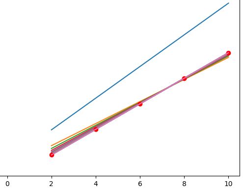
As you can see the first guess is WAY off because the Neural Network has nothing to go off of, but those clever machines learn quickly and you can see how fast it hones in on the right answer.
The full code
If you’re looking for the full code you can –> click here <–